
Fracking Boom Gives Banks Mortgage Headaches
November 15, 2013Next Up For Pope Francis: Anti-Fracking Activist?
November 17, 2013Here is a lot of information on Marcellus shale decline rates
SCROLL DOWN: The impact of high decline rates on the economics of gas drilling is huge. Companies are pulling out of the Marcellus due to poor profitability prospects.
Arthur Berman first calculated the decline rates in 2009 – once public, the companies could not lie to their stockholders – they sort of tried to hide it on page 10, but… we noticed!

The decline rates reported by Chesapeake Energy mean that a gas field with 5 wells initially must have 3 new wells drilled each and every year, after the first year, in order to simply maintain the production of the original 5 wells (see our analysis). A field with 100 wells initially must have 60 new wells drilled every year just to maintain production.
In order to increase production every year (blue Cumulative Production curve above), a gas field must be constantly expanded every year going forward. So much damage, and for what?
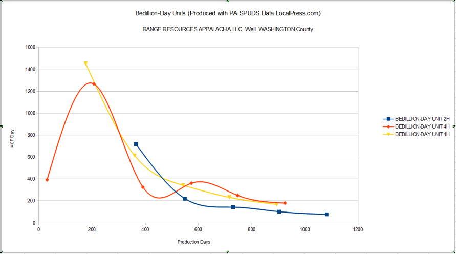
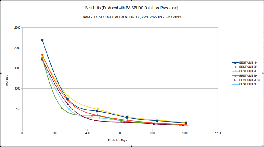
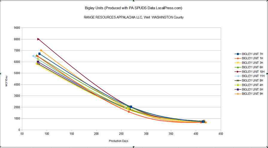
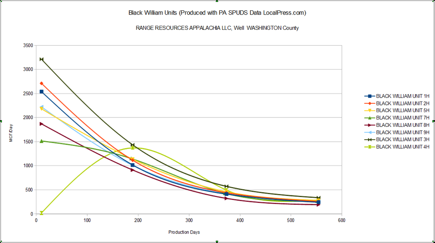
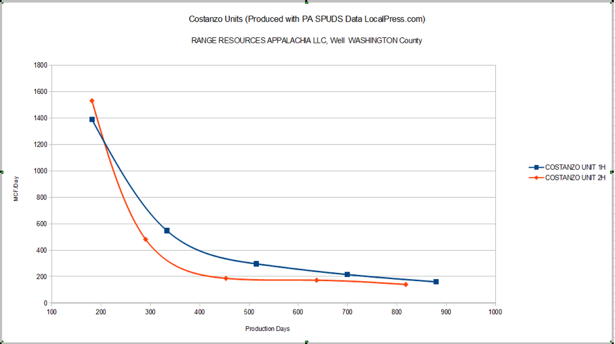
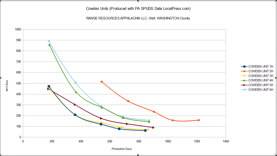
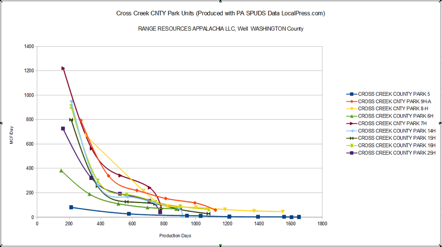
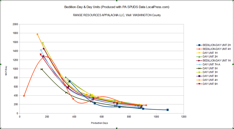
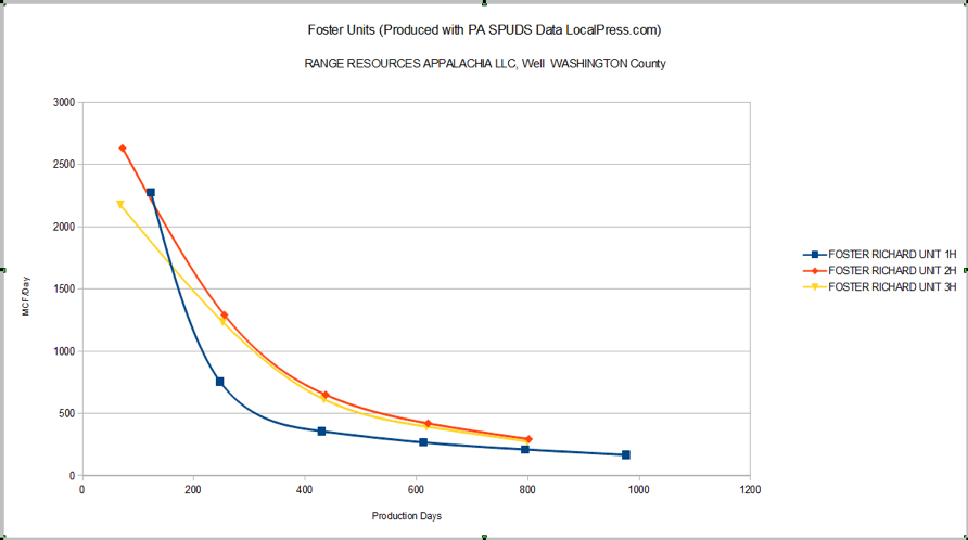
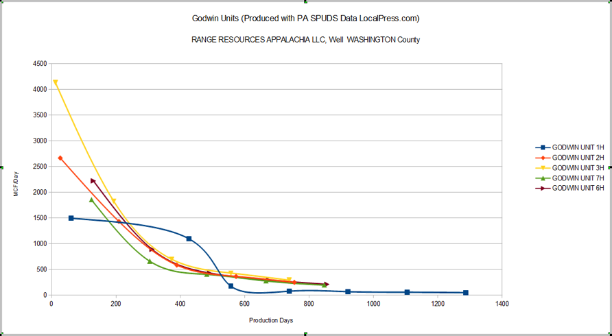
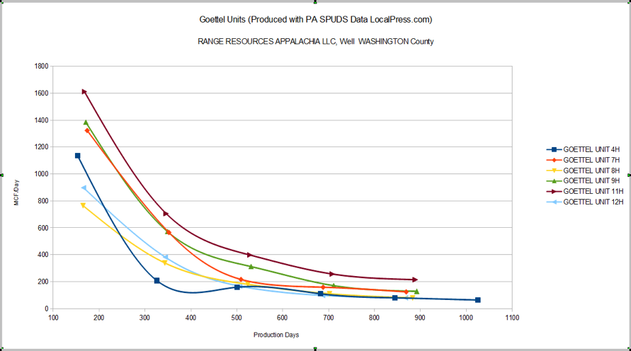
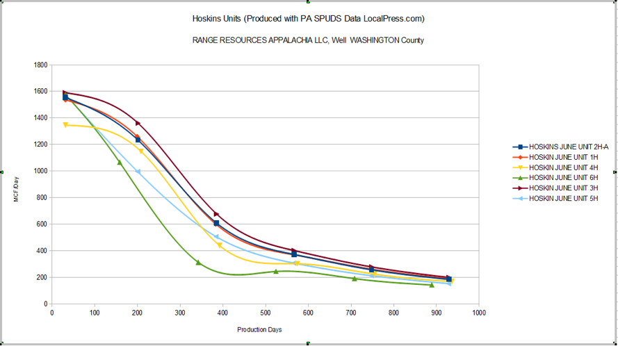
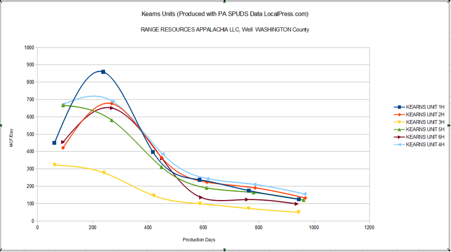
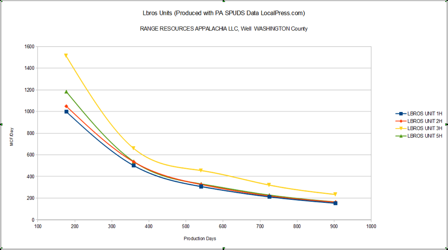
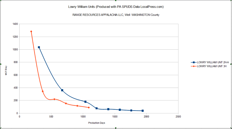
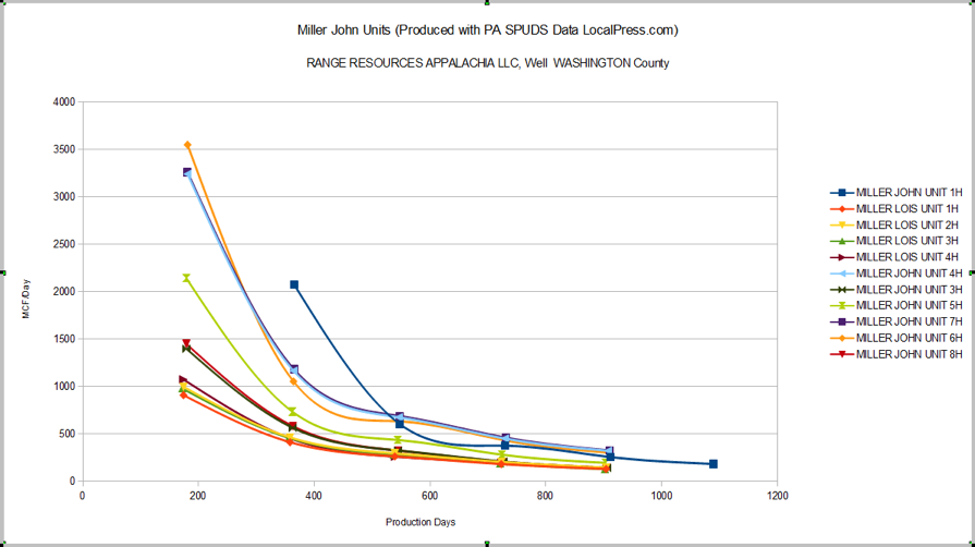
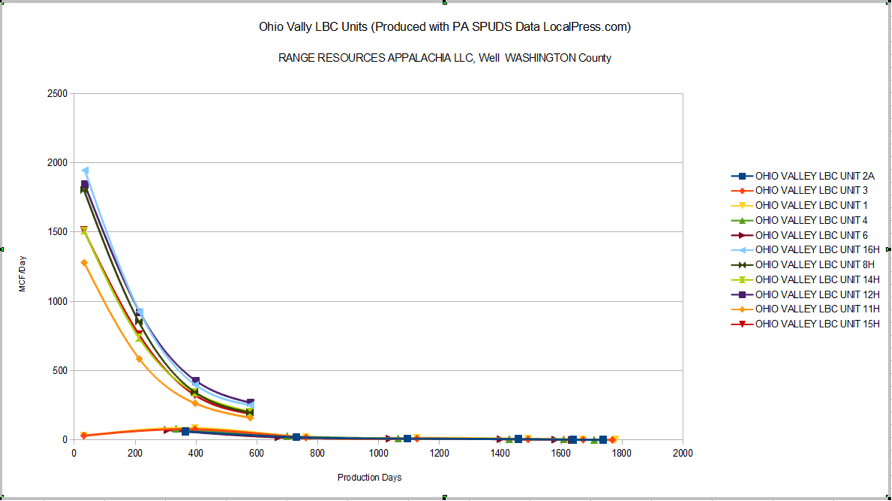
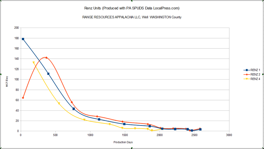
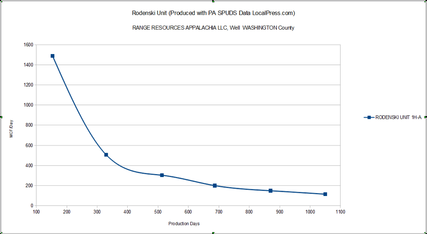
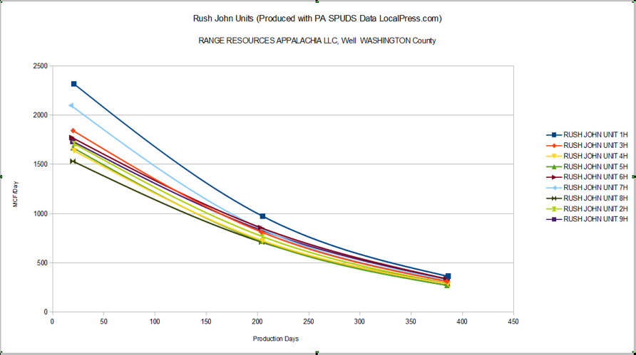
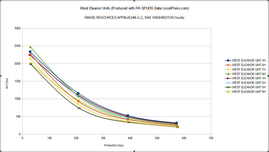
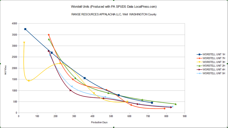
The following graphs and information are from contributions by Leland T. Snyder (see SPUDS Access for data) and Bob Donnan, as noted. All are based on data from the PA DEP. Actual data from western PA Marcellus wells “points to a 65-percent drop in production over the first 3 years, with further declines of 8 percent per year after that.” Production drops more where there is only dry gas (no liquids), as in northeast PA.
Bob Donnan has “tracked 190 wells at over three dozen drilling locations with actual Marcellus gas well production numbers, to clearly show how much gas has been produced, and more importantly, how much gas production has declined over the first years of shale gas production.” Scroll down his page to see individual Marcellus shale well data.
The industry is aware of these decline rates, as shown by the Chesapeake graph above and this industry study (from Schlumberger) of the Barnett, Fayetteville, Woodford and Haynesville gas fields.
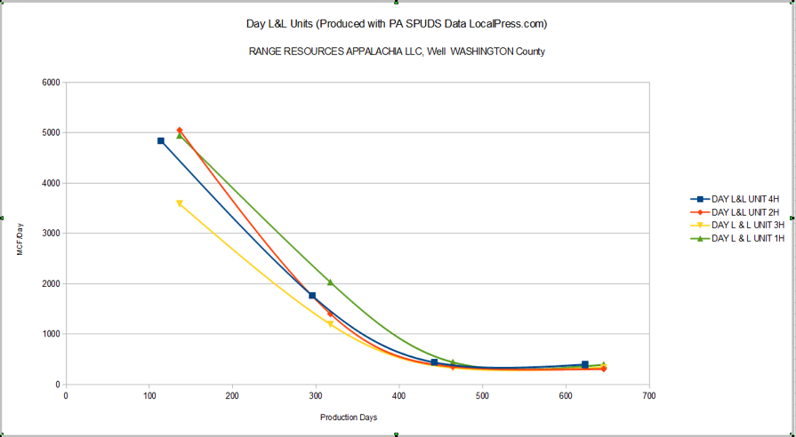
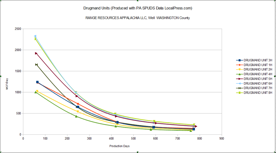
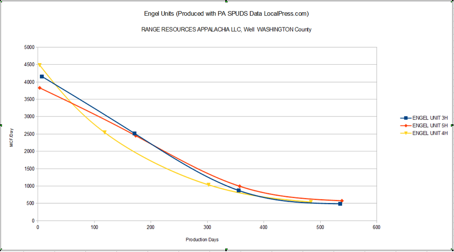
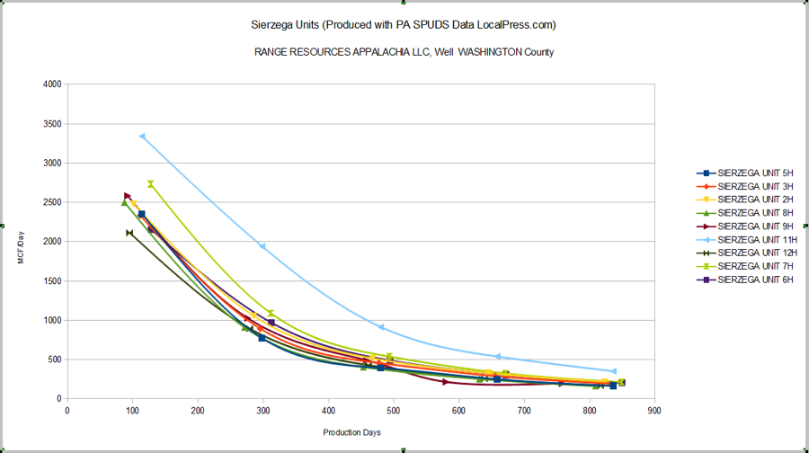
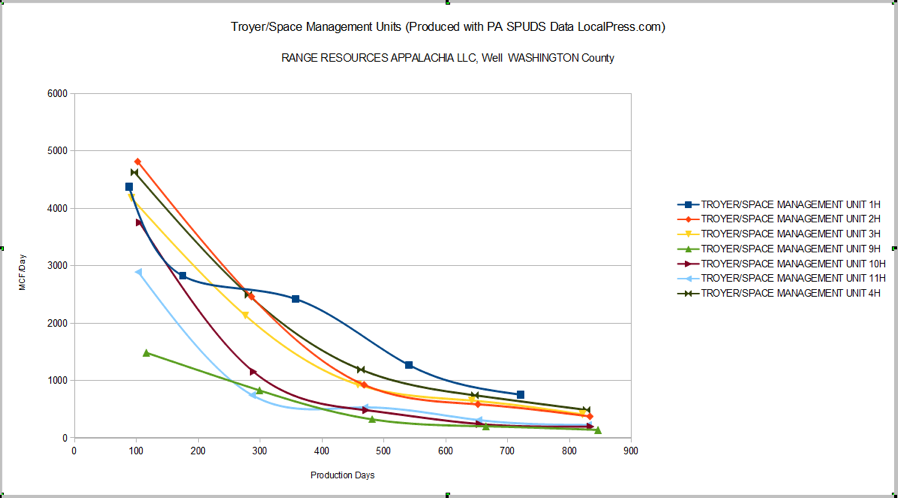
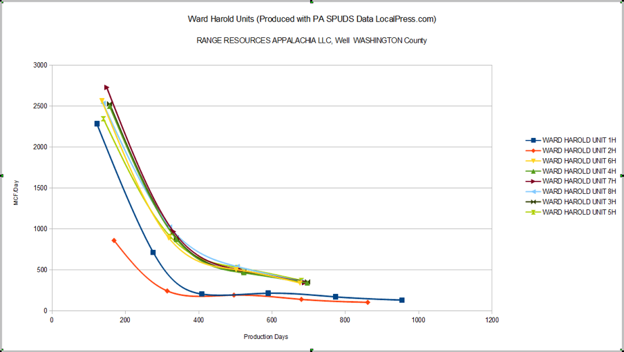
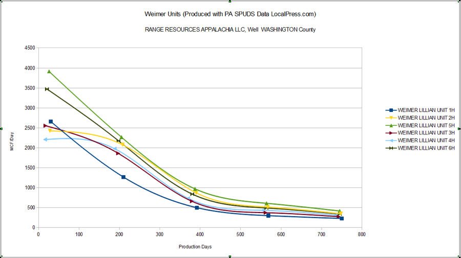
The following graphs show production data (vertical axis) for individual wells over time (horizontal axis). Production data is either in cubic feet per day or thousand cubic per day (MCF/Day). Time is in days. Note: The scale on the graphs varies. There will be further additions to the information on this page.

Data for Cabot wells (dry gas) in northeast PA
Note: Wells without a steep decline curve had low initial production.
The following graphs are from western PA, except for the last one.


Data for XTO Energy wells in northeast PA
Note: The best XTO Energy wells in Lycoming County had initial production of about 4 million cubic feet per day as compared to the best Cabot wells in northeast PA (near top) which had initial production of about 11 million cubic feet per day. The XTO wells are not high producing wells.


For more information, see Marcellus-Shale.us by Bob Donnan.